Stat-Ease Blog

Keep your experiment planned, but random

When I wrote my introduction to factorial design (Greg’s DOE Adventure - Factorial Design, Part 1), there were a couple of points that I left out. I’ll amend that post here to talk about making sure your experiment is planned out yet random.

Wait. What?

You’ll see. Let me explain.

Getting organized

During the initial phase of an experiment, you should make sure that it is well planned out. First, think about the factors that affect the outcome of your experiment. You want to create a list that’s as all-encompassing as possible. Anything that may change the outcome, put on your list. Then pare it down into the ones that you know are going to be the biggest contributors.

Once you have done that, you can set the levels at which to run each factor. You want the low and high levels to be as far apart as possible. Not too low that you won’t see an effect (if your experiment is cooking something, don’t set the temperature so low that nothing happens). Not too high that it’s dangerous (as in cooking, you don’t want to burn your product).

Finally, you want to make sure your experiment is balanced when it comes to the factors in your experiment. Taking the cooking example above a little further, suppose you have three factors you are testing: time, temperature, and ingredient quality. Let’s also say that you are testing at two different levels: low and high (symbolized by minus and plus signs, respectively). We can write this out in a table:

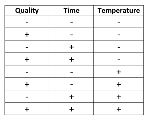
This table contains all the possible combinations of the three factors. It’s called an ‘orthogonal array’ because it’s balanced. Each column has the same number of pluses and minuses (4 in this case). This balance in the array allows all factors to be uncorrelated and independent from each other.

With these steps, you have ensured that your experiment is well planned out and balanced when looking at your factors.

Always randomize

At the start of this post, I said that an experiment should be planned out, yet random. Well we have the planned-out part, now let’s get into the random part.

In any experimentation, influence from external sources (variables you are not studying) should be kept to a minimum. One way to do this is randomizing your runs.

As an example, let’s look at the table above with the cooking example. Let’s say that it represents the order of how the experiment was run. So, all the low temperature runs were made together and then all the high ones together. This makes sense, right? Perform all the runs at one temperature before adjusting up to the next setting.

The problem is, what if there is an issue with your oven that causes the temperature to fluctuate more, early in the experiment and less later. This time-related issue introduces variation (bias) into your results that you didn’t know about.

To reduce the influence of this variable, randomize your run order. It may take more time adjusting your oven for every run, but it will remove that unwanted variation.

Temperature is a popular example to illustrate randomization. But this can be said of any factor that may have time-related problems. It could be warm-up time on a machine or the physical tiring of an operator. Randomization is used to guard against bias as much as you can when running an experiment.

Conclusions

Hopefully, you see now why I said to keep your experiments planned but random. It sounds like an oxymoron, but it’s not. Not in the way I’m talking about it here!

So, I’ve gotten thru some of the basics (Greg's DOE Adventure: Important Statistical Concepts behind DOE and Greg’s DOE Adventure - Simple Comparisons). These are the ‘building blocks’ of design of experiments (DOE). However, I haven’t explored actual DOE. I start today with factorial design.

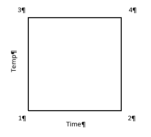
In this case, the horizontal line (x-axis) is time and vertical line (y-axis) is temperature. The area in the box formed is called the Experimental Space. Each corner of this box is labeled as follows:

1 – low time, low temperature (resulting in crunchy, matchstick-like pasta), which can be coded minus-minus (-,-)

2 – high time, low temperature (+,-)

3 – low time, high temperature (-,+)

4 – high time, high temperature (making a mushy mass of nasty) (+,+)

One takeaway at this point is that when a test is run at each point above, we have 2 results for each level of each factor (i.e. 2 tests at low time, 2 tests at high time). In factorial design, the estimates of the effects (that the factors have on the results) is based on the average of these two points; increasing the statistical power of the experiment.

If we look at the same experiment from the perspective of altering just one factor at a time (OFAT), things change a bit. In OFAT, we start at point #1 (low time, low temp) just like in the Factorial model we just outlined (illustrated below).

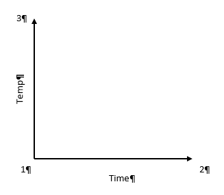
Here, we go from point #1 to #2 by lengthening the time in the water. Then we would go from #1 to #3 by changing the temperature. See how this limits the number of data points we have? To get the same power as the Factorial design, the experimenter will have to make 6 different tests (2 runs at each point) in order to get the same power in the experiment.

After seeing these results of Factorial Design vs OFAT, you may be wondering why OFAT is still used. First of all, OFAT is what we are taught from a young age in most science classes. It’s easy for us, as humans, to comprehend. When multiple factors are changed at the same time, we don’t process that information too well. The advantage these days is that we live in a computerized world. A computer running software like Design-Expert®, can break it all down by doing the math for us and helping us visualize the results.

Additionally, with the factorial design, because we have results from all 4 corners of the design space, we have a good idea what is happening in the upper right-hand area of the map. This allows us to look for interactions between factors.

That is my introduction to Factorial Design. I will be looking at more of the statistical end of this method in the next post or two. I’ll try to dive in a little deeper to get a better understanding of the method.

As I learn about design of experiments, it’s natural to start with simple concepts; such as an experiment where one of the inputs is changed to see if the output changes. That seems simple enough.

For example, let’s say you know from historical data that if 100 children brush their teeth with a certain toothpaste for six months, 10 will have cavities. What happens when you change the toothpaste? Does the number with cavities go up, down, or stay the same? That is a simple comparative experiment.

“Well then,” I say, “if you change the toothpaste and 6 months later 9 children have cavities, then that’s an improvement.”

Not so fast, I’m told. I’ve already forgotten about that thing called variability that I defined in my last post. Great.

In that first example, where 10 kids got cavities. That result comes from that particular sample of 100 kids. A different sample of 100 kids may produce an outcome of 9, other times it’s 11. There is some variability in there. It’s not 10 every time.

[Note: You can and should remove as much variability as you can. Make sure the children brush their teeth twice a day. Make sure it’s for exactly 2 minutes each time. But there is still going to be some variation in the experiment. Some kids are just more prone to cavities than others.]

How do you know when your observed differences are due to the changes to the inputs, and not from the variation?

It’s called the F-Test.

I’ve seen it written as:

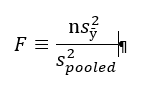
Where:

s = standard deviation

s2 = variance

n = sample size

y = response

ӯ (“y bar”) = average response

In essence, this is the amount of variance for individual observations in the new experiment (multiplied by the number of observations) divided by the total variation in the experiment.

Now that, by itself, does not mean much to me (see disclaimer above!). But I was told to think of it as the ratio of signal to noise. The top part of that equation is the amount of signal you are getting from the new condition; it’s the amount of change you are seeing from the established mean with the change you made (new toothpaste). The bottom part is the total variation you see in all your data. So, the way I’m interpreting this F-Test is (again, see disclaimer above): measuring the amount of change you see versus the amount of change that is naturally there.

If that ratio is equal to 1, more than likely there is no difference between the two. In our example, changing the toothpaste probably makes no difference in the number of cavities.

As the F-value goes up, then we start to see differences that can likely be credited to the new toothpaste. The higher the value of the F-test, the less likely it is that we are seeing that difference by chance and the more likely it is due to the change in the input (toothpaste).

Trivia

Question: Why is this thing called an F-Test?

Answer: It is named after Sir Ronald Fisher. He was a geneticist who developed this test while working on some agricultural experiments. “Gee Greg, what kind of experiments?”. He was looking at how different kinds of manure effected the growth of potatoes. Yup. How “Peculiar Poop Promotes Potato Plants”. At least that would have been my title for the research.

If you read my previous post, you will remember that design of experiments (DOE) is a systematic method used to find cause and effect. That systematic method includes a lot of (frightening music here!) statistics.

[I’ll be honest here. I was a biology major in college. I was forced to take a statistics course or two. I didn’t really understand why I had to take it. I also didn’t understand what was being taught. I know a lot of others who didn’t understand it as well. But it’s now starting to come into focus.]

Before getting into the concepts of DOE, we must get into the basic concepts of statistics (as they relate to DOE).

Basic Statistical Concepts:

Variability
In an experiment or process, you have inputs you control, the output you measure, and uncontrollable factors that influence the process (things like humidity). These uncontrollable factors (along with other things like sampling differences and measurement error) are what lead to variation in your results.

Mean/Average
We all pretty much know what this is right? Add up all your scores, divide by the number of scores, and you have the average score.

Normal distribution
Also known as a bell curve due to its shape. The peak of the curve is the average, and then it tails off to the left and right.

Variance
Variance is a measure of the variability in a system (see above). Let’s say you have a bunch of data points for an experiment. You can find the average of those points (above). For each data point subtract that average (so you see how far away each piece of data is away from the average). Then square that. Why? That way you get rid of the negative numbers; we only want positive numbers. Why? Because the next step is to add them all up, and you want a sum of all the differences without negative numbers getting in the way. Now divide that number by the number of data points you started with. You are essentially taking an average of the squares of the differences from the mean.

That is your variance. Summarized by the following equation:

In this equation:

Yi is a data point
Ȳ is the average of all the data points
n is the number of data points

Standard Deviation
Take the square root of the variance. The variance is the average of the squares of the differences from the mean. Now you are taking the square root of that number to get back to the original units. One item I just found out: even though standard deviations are in the original units, you can’t add and subtract them. You have to keep it as variance (s2), do your math, then convert back.

Hi there. I’m Greg. I’m starting a trip. This is an educational journey through the concept of design of experiments (DOE). I’m doing this to better understand the company I work for (Stat-Ease), the product we create (Design-Expert® software), and the people we sell it to (industrial experimenters). I will be learning as much as I can on this topic, then I’ll write about it. So, hopefully, you can learn along with me. If you have any comments or questions, please feel free to comment at the bottom.

So, off we go. First things first.

What exactly is design of experiments (DOE)?

When I first decided to do this, I went to Wikipedia to see what they said about DOE. No help there.

The what now?

That’s not what I would call a clearly conveyed message. After some more research, I have compiled this ‘definition’ of DOE:

Obviously, that works for me since I wrote it. But does it work for you?

So, conceptually I’m off and running. But why do we need ‘designed experiments’? After all, isn’t all experimentation about combining some inputs, measuring the outputs, and looking at what happened?

The key words above are ‘systematic method’. Turns out, if we stick to statistical concepts we can get a lot more out of our experiments. That is what I’m here for. Understanding these ‘concepts’ within this ‘systematic method’ and how this is advantageous.

Well, off I go on my journey!