Stat-Ease Blog

Categories
Thinking Outside the Box by Using Standard Error to Constrain Optimization
Response surface methods (RSM) pave the way to the pinnacle of process improvement. However, the central composite design (CCD)—the most common layout for RSM (pictured in Figure 1 for three factors)—traditionally limits the region of prediction to the cubical core. This conservative view avoids dangerous extrapolation out to the far reaches of the space defined by the axial ranges of the star points. This article lays out a less-limiting (but still reasonably safe) approach to optimization based on using a specified standard error (SE) of prediction as the boundary for searching out the optimal process setup.
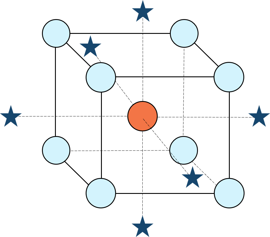
Figure 1: Central composite design for three factors
Three different methods for defining the search area will be detailed for a four-factor CCD. The goal is to avoid extrapolating beyond where the data provides adequate knowledge about the response while maximizing the volume that will be explored.
Let’s compare three boundaries for defining the search area in the factor space, the first two of which do not make use of the SE:
1. Factorial bounded—the hypercube* with vertices at coded values ±1, thus each edge spans 2 coded units. The volume of this four-dimensional hypercube is 16 (=2x2x2x2). The maximum SE is 0.764, which occurs at the vertices (i.e., corners). See figure 2. For comparison’s sake, we will use this SE (0.764) as our benchmark—anything more than this will be deemed unacceptable.
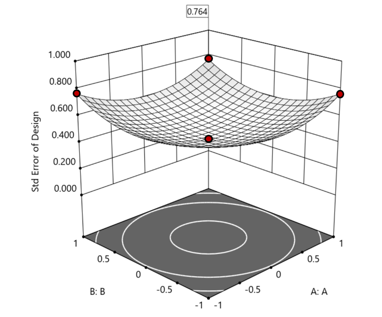
Figure 2. Looking only at the factorial region (±1), with factors C and D set to +1, we see that the highest SE values observed are at the factorial corners.
2. Axial (star-point) bounded—a cube with vertices at ±2 to include the star runs.
The volume of this four-dimensional hypercube is huge: 256 coded units (=4x4x4x4), which offers big advantages for optimization. However, most of the volume (69%) exhibits an SE ≥ 0.764 (maximum is 2.963!). Therefore, this method must be rejected. See figure 3.
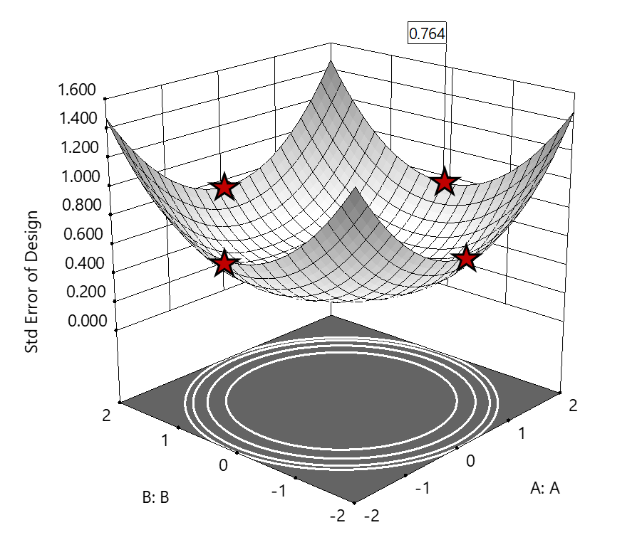
Figure 3. The default axial point placement is at ±2, which for 4 factors creates a rotatable design. The axial points therefore have the same SE as the factorial corner points—all are equidistant from the center. Note that factors C and D are set to zero (center) and the range for factors A and B are increased to ±2 to show the axial points.
3. Standard error bounded—the area within SE ≤0.764.*
Once again looking at figure 3, the SE at the axial (star) points equals that of the ±1 factorial points. Limiting the standard error ≤0.764 produces a hypersphere with a radius of 2. The volume of this hypersphere is 78.96, almost five times larger than the ±1 factorial hypercube.
Summarizing the three methods of defining the search area in the factor space:
- The factorial cube with vertices at ±1 may be too restrictive and may not include all the volume where acceptable predictions could be made.
- A cube with vertices at ±2 that includes the axial runs is too liberal; most of the volume has poor predictions.
- Defining the search area by standard error may prove insightful—it includes all the areas where acceptable predictions may reside.
Using standard error to constrain the optimization defines a search area that matches its properties:
- Spheres for rotatable CCDs. (Note: The above graphics and discussion assumed the choice of alpha values produced a spherical standard error plot).
- Cubes for face-centered CCDs.
- Irregular shapes for central composite designs with alpha between 1 and that recommended for rotatable designs, optimal designs, models for which model reduction was applied, and historical data.
An added bonus to using SE is that it adjusts the search area for reduced models and/or missing data.
It should be noted that it is assumed the design was sized for precision and contains enough data to make sound predictions within the cube (or hypercube). If the FDS is low (for example, below 80%), then making good predictions within the cube is already challenged. Extending the search zone outside the cube would exacerbate things further.
Another caveat is the assumption that a quadratic model pertains outside the design cube. The primary purpose of axial points in a central composite design is to fortify the estimates of quadratic terms to be applied within the cube. Sometimes the specified quadratic model performs well inside the cube, but extrapolation becomes dangerous due to higher-order behavior beyond the faces of the cube. Checking the diagnostic plots for anomalous behavior of the axial points can provide some assurance that the quadratic model is useful beyond the cube.
So, the key takeaway is this. Adding standard error to the search criteria and expanding the factor ranges beyond the edges of the factorial cube can be helpful for making judicious extrapolations beyond the edges of the cube. Simply applying the highest standard error found within the cube to regions outside the cube is a reasonable place to start, especially when the FDS performance of the design is over 80%. It is advisable to treat any interesting discoveries as tentative until verified by confirmation runs, augmented designs, or an entirely new design focused on the projected area of interest.
For more information on how to include standard error in the optimization module, see: Extrapolating a Response Surface Design in the Stat-Ease software Help menu.
*For 3 factors we can envision the factorial design space as a cube. With more than 3 factors (in this case 4 factors) we refer to the analogous region as a hypercube.
Acknowledgement: This post is an update of an article by Pat Whitcomb of the same title, published in the April 2017 STATeaser.
Like the blog? Never miss a post - sign up for our blog post mailing list.
The Importance of Center Points in Central Composite Designs
A central composite design (CCD) is a type of response surface design that will give you very good predictions in the middle of the design space. Many people ask how many center points (CPs) they need to put into a CCD. The number of CPs chosen (typically 5 or 6) influences how the design functions.
Two things need to be considered when choosing the number of CPs in a central composite design:
1) Replicated center points are used to estimate pure error for the lack of fit test. Lack of fit indicates how well the model you have chosen fits the data. With fewer than five or six replicates, the lack of fit test has very low power. You can compare the critical F-values (with a 5% risk level) for a three-factor CCD with 6 center points, versus a design with 3 center points. The 6 center point design will require a critical F-value for lack of fit of 5.05, while the 3 center point design uses a critical F-value of 19.30. This means that the design with only 3 center points is less likely to show a significant lack of fit, even if it is there, making the test almost meaningless.
TIP: True “replicates” are runs that are performed at random intervals during the experiment. It is very important that they capture the true normal process variation! Do not run all the center points grouped together as then most likely their variation will underestimate the real process variation.
2) The default number of center points provides near uniform precision designs. This means that the prediction error inside a sphere that has a radius equal to the ±1 levels is nearly uniform. Thus, your predictions in this region (±1) are equally good. Too few center points inflate the error in the region you are most interested in. This effect (a “bump” in the middle of the graph) can be seen by viewing the standard error plot, as shown in Figures 1 & 2 below. (To see this graph, click on Design Evaluation, Graph and then View, 3D Surface after setting up a design.)
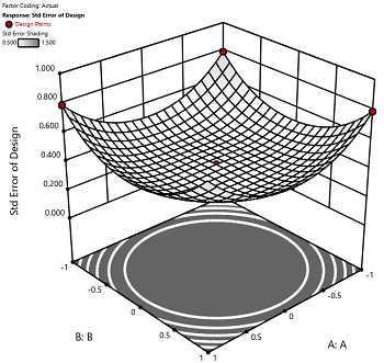
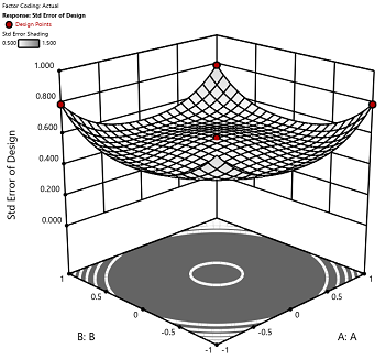
Figure 1 (left): CCD with the 6 center points (5-6 recommended). Figure 2 (right): CCD with only 3 center points. Notice the jump in standard error at the center of figure 2.
Ask yourself this—where do you want the best predictions? Most likely at the middle of the design space. Reducing the number of center points away from the default will substantially damage the prediction capability here! Although it can seem tedious to run all of these replicates, the number of center points does ensure that the analysis of the design can be done well, and that the design is statistically sound.