R-Squared Mysteries Solved

Design of experiments (DOE) and the resulting data analysis yields a prediction equation plus a variety of summary statistics. A set of R-squared values are commonly used to determine the goodness of model fit. In this blog, I peel back the raw versus adjusted versus predicted R-squared and explain how each can be interpreted, along with the relationships between them. The calculations of these values can be easily found online, so I won’t spend time on that, focusing instead on practical interpretations and tips.

Raw R-squared measures the fraction of variation explained by the fitted predictive model. This is a good statistic for comparing models that all have the same number of terms (like comparing models consisting of A+B versus A+C). The downfall of this statistic is that it can be artificially increased simply by adding more terms to the model, even ones that are not statistically significant. For example, notice in Table 1 from an optimization experiment how R-squared increases as the model steps up in order from linear to two-factor interaction (2FI), quadratic and, finally, cubic (disregarding it being aliased).

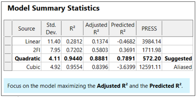
The “adjusted” R-squared statistic corrects this ‘inflation’ by penalizing terms that do not add statistical value. Thus, the adjusted R-squared statistic generally levels off (at 0.8881 in this case) and then begins to decrease at some point as seen in Table 1 for the cubic model (0.8396). The adjusted R-squared value cannot be inflated by including too many model terms. Therefore, you should report this measure of model fit, not the raw R-squared.

The “predicted” R-squared is most rigorous for assessing model fit, so much so that it often starts off negative at the linear order, as it does for the example in Table 1 (-0.4682). As you can see, this statistic improves greatly as significant terms are added to the model, and quickly decreases once non-significant terms are added, e.g., going negative again at cubic. If predicted R-squared goes negative, the model becomes worse than nothing, that is, simply taking the average of the data (a “mean” model)—that is not good!

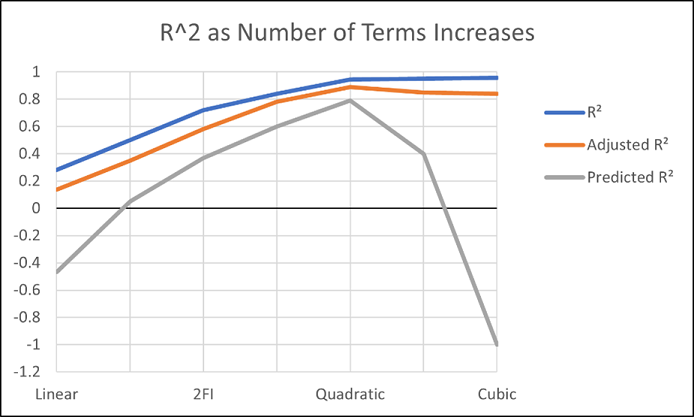
Figures 1 illustrates how the predicted R-squared peaks at the quadratic model for the example. Once a model emerges at the highest adjusted and/or predicted R-squared, consider taking out any insignificant terms—best done with the aid of a computerized reduction algorithm. This often produces a big increase in the predicted R-squared.

Conclusion

The goal of modeling data is to correctly identify the terms that explain the relationship between the factors and the response. Use the adjusted R-squared and predicted R-squared values to evaluate how well the model is working, not the raw R-squared.

PS: You’ve likely been reading this expecting to find recommended adjusted and predicted R-squared values. I will not be providing this. Higher values indicate that more variation in the data or in predictions is explained by the model. How you use the model dictates the threshold that is acceptable to you. If the DOE goal is screening, low values can be acceptable. Remember that low R-squared values do not invalidate significant p-values. In other words, if you discover factors that have strong effects on the response, that is positive information, even if the model doesn’t predict well. A low predicted R-squared means that there is more unexplained variation in the system, and you have more work to do!