Improving Your Predictive Model via a Response Transformation
A good predictive model must exhibit overall significance and, ideally, insignificant lack of fit plus high adjusted and predicted R-squared values. Furthermore, to ensure statistical validity (e.g., normality, constant variance) the model’s residuals must pass a series of diagnostic tests (fortunately made easy by Stat-Ease software):
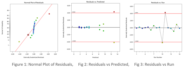
- Normal plot of residuals illustrates a relatively straight line. If you can cover the residuals with a fat pencil, no worries, but watch out for a pronounced S-shaped curve such as Figure 1 exhibits.
- Residuals-versus-predicted plot has points scattered randomly, i.e., demonstrating a constant variance from left to right. Beware of a “megaphone” shape as seen in Figure 2.
- Residuals-versus-run plot exhibiting no trends, shifts or outliers (points outside the red lines such as seen in Figure 3).
When diagnostic plots of residuals do not pass the tests, the first thing you should consider for a remedy is a response transformation, e.g., rescaling the data via a natural log (again made easy by Stat-Ease software). Then re-fit the model and re-check the diagnostic plots. Often you will see improvements in both the statistics and the plots of residuals.
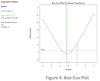
The Box-Cox plot (see Figure 4) makes the choice of transformation very simple. Based on the fitted model, this diagnostic displays a comparable measure of residuals against a range of power transformations, e.g., taking the inverse of all your responses (lambda -1), or squaring them all (lambda 2). Obviously, the lower the residuals the better. However, only go for a transformation if your current responses at the power of 1 (the blue line), fall outside the red-lined confidence interval, such as Figure 4 display. Then, rather than going to the exact-optimal power (green line), select one that will be simpler (and easier to explain)--the log transformation in this case (conveniently recommended by Stat-Ease software).
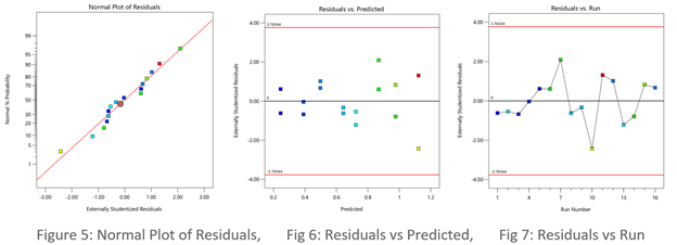
See the improvement made by the log transformation in the diagnostics (Figures 5, 6 and 7). All good!
In conclusion, before pressing ahead with any model (or abandoning it), always check the residual diagnostics. If you see any strange patterns, consider a response transformation, particularly if advised to do so by the Box-Cox plot. Then confirm the diagnostics after re-fitting the model.
For more details on diagnostics and transformations see How to Use Graphs to Diagnose and Deal with Bad Experimental Data.
Good luck with your modeling!
~ Shari Kraber, shari@statease.com